This project was done with colleague Goran Popović.
Project idea
The aim of this project was to design, construct and test a device that would serve as a phone book for landline phones. The device is connected between the phone and the phone line and therefore can serve as a memory for phone numbers. It is important that it has a very simple interface and allows unobstructed use of the phone. The device was tested by visually impaired people and feedback showed that it could be used without any problem and without special training.
—————————————————————————————————————————————–
Motivation
Long distance communication has become a crucial part of life of the modern man. Without the Internet it is difficult to perform even simple personal tasks, but without phone it is almost impossible. The emergence of the SMS has brought a whole new dimension of life to the hearing impaired persons.
At the first sight phones make communication of blind people easier, but only seemingly. In fact, in everyday life we use dozens, even hundreds of phone numbers. It is almost impossible to know them by heart. Today most of the people remember only a few phone numbers which they call frequently because they rely on the phonebook in their mobile phones where phone numbers are stored. Blind people do not have a possibility to write the number on the paper, nor in the mobile phones (most of them). Some people record phone numbers on audio cassettes or CDs in order to have a sort of an audio phonebook, and some, albeit rare have phone numbers written in Braille.
It is a myth that blind people, because of blindness have an excellent memory. This actually applies only to those who are systematically working to develop their mnemonics. Just like in the general population, among blind people exists a significant number of those who are not skilled with technical devices as well as those with poor memory skills. To these people it is a problem to call more than a few different phone numbers.
Based on research of Internet and scientific publications as well as consulting with blind people and their associations, it was concluded that today there is no available device that solves this problem. Also, almost all devices that are suitable for the blind (like speaking clocks, scales, blood pressure monitors, etc.) are several times more expensive [1] than the same devices for people who can see. Most of the devices are also even more expensive if the language of the device is not English.
The two biggest problems that blind people have are calling the wrong number and the fact that the call is interrupted due to the long pause between entering two digits (more than eight seconds). Wrong number is entered mainly due to inadequate phone interfaces for blind people. Interruption of the call happens because people often must look for a phone number in their own phonebooks.
The aim of this project was to solve this problem.
Idea of the project
The hypothesis is that this problem can be solved by constructing a device that can be connected between phone device and phone landline that would serve as an audio phonebook. It would have just about three buttons in order to be easy to operate. Buttons would enable scrolling through contacts which would be pronounced (the contact’s name) and automatically dialed by pressing the “dial” button once the desired contact is found.
Such device would allow blind people much easier and faster handling with the telephone device. One needs to type the phone number only once, in order to program the phonebook, which greatly facilitates the use, since there is no need to remember a lot of numbers, nor for creating any alternative phonebooks. On the other hand ordinary phones, often because of inadequate interfaces (like a lot of small buttons that are inadequately positioned) make entering the phone numbers difficult. The proposed device would reduce the use of phone keys to a minimum.
The second hypothesis is that such audio phonebook would eliminate wrong calls which are today present due to false memory or mistakes in operating the phone keys. The third hypothesis is that the audio phonebook could be used also by people with reduced cognitive and motor abilities.
Existing solutions to the problem
Research has shown that there are two main groups of solutions to this problem: alternative phonebooks and mobile phones.
1.Alternative phonebooks
Auxiliary phonebooks that blind people use are usually CDs, audio cassettes or notes/address books in Braille which contain contact’s information. Usage of any of the mentioned phonebooks is very slow and clumsy.
The phones with big buttons or with Braille labels can be bought, but still the problem of remembering a phone number is not resolved because the landline phones have a small memory: 10, 20 or 30 numbers. Even if such phones would have a larger memory, the problem is remembering at which memory location is the desired number, and there is no feedback except waiting for who will answer the call. In some countries the law requires that manufacturers of phone equipment need to produce devices that are adapted for the blind, visually impaired, deaf or people with other disabilities, but the requirements that need to be fulfilled are usually minimal.
2.Mobile phone solutions
Blind people have several feasible ways to call a large number of different phone numbers, but they are adapted for people with advanced technical competences: mobile phones with talkback and mobile phones with voice recognition.
Mobile phone with talkback has a program running in the background that pronounces screen’s content [2]. With that program blind user can select a phonebook, and find the desired contact. The advantage of this solution is that it uses existing, conventional models of phones (“smartphones”), phonebook size is practically unlimited, and the additional cost is only for the voice program. The disadvantage is that coping with a multitude of programs available on mobile phone, without tactile (and visual) feedback, is cognitively very demanding, and requires intense training which can be very hard to overcome for many people.
Phonebook with voice recognition [3] appeared on mobile phones even before the era of smartphones, and it is also accomplished by means of a computer program on a mobile phone. The advantages are the unlimited number of contacts, any phone can be used and the cost is only for getting certain programs. The disadvantage is that such programs do not yet have a high level of recognition, so it is necessary to use very distinguishable names of the contacts: words that do not sound similar.
None of the available methods is suitable for all blind people, especially the elderly people who recently got blind or people with reduced motor and cognitive abilities.
Concept and requirements for the device
1.Required functionalities
One of the main requirements is that the device does not limit the usage of phones and phone lines, regardless of the state of the device. This means that users can still make a phone call or answer an incoming call as if the device is not connected. Another requirement is the ability to save a large number of contacts (several hundred). Also, the user must be able to enter a new contact without anybody’s help, at any time and at any position in the phonebook as he prefers. This means that moving, deleting and adding new contact anywhere in the phonebook must be possible.
The basic functionality is pronouncing the name of the contact that is selected. It is also important to be able to hear the phone number that is stored under each of the contacts. To use these options (finding the desired contact, adding a new contact, moving contact and deleting the contact) device must have voice instructions that guide the user through each function. Also, if there are a large number of contacts in the phonebook, functionality of rapid search is required and phonebook must be circularly shaped: after the last contact, comes the first, and vice versa.
2.User interface requirements
Several functions are mentioned that phonebook must have. For this reason, in order for operation to be simple, it is important that steps for each implemented functionality are logic and intuitive. Also, the physical interface must be easy to use.
The goal was to create a device with as few buttons as possible. Most important operation is „listing“, but also other operations such as calling, accepting and rejecting (e.g. just recorded name of the contact or entered phone number) and exiting (e.g. out of current option) are needed during the use of the device. All of operations can be implemented with one button, by different number of clicks on the button (one, two or three clicks). In such a way a total number of buttons can be reduced to only three buttons or even only one if encoder knob, which can be rotated and pressed, is used.
3.Flexibility requirements
Except mentioned functionalities, the goal is also that the device can be easily translated into any language. Contact names need no translation since they are entered by the user in the language he prefers. The only thing that needs to be translated into another language, are voice instructions that guide the user through the functionalities of the device. These voice instructions, as well as all the contacts, are stored on the SD memory card. Voice instructions are files in WAV format that can be recorded on any personal computer in a matter of minutes. In the same way contacts can be quickly and massively recorded, which is useful when initially storing a lot of contacts in an empty phonebook. This requires a separate program for the personal computer, for which a help of a sighted person is needed.
In addition, the goal is that the device is as cheap as possible and can be built by anyone. Therefore, the device is based on “open source” hardware so later anyone could make it, even the ones who have no engineering skills.
Device development
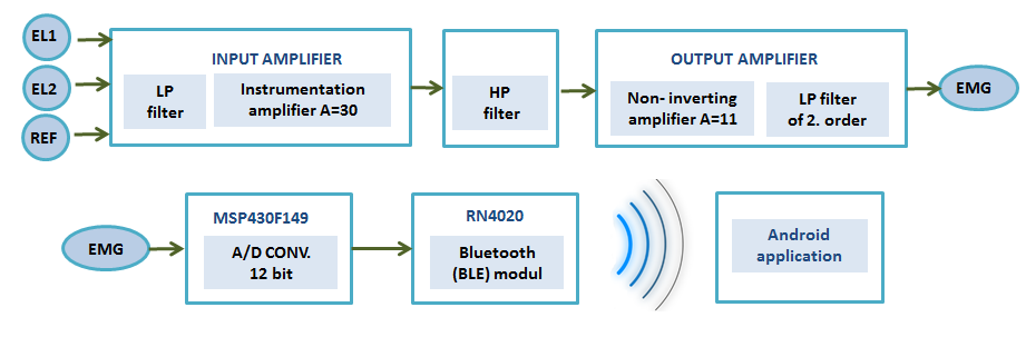
1.Hardware
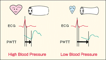
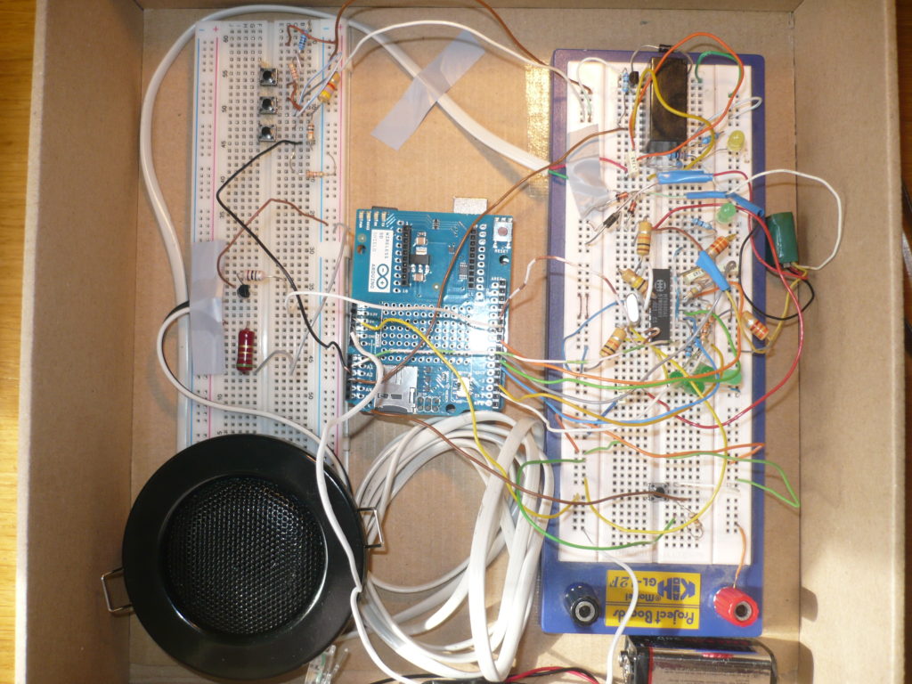
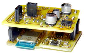
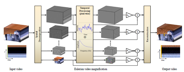
General parts of the device are Arduino [5], DTMF encoder/decoder [6], speaker, microphone, memory (SD card), power supply, and the control circuit for the phone line as shown in figure below. The device is connected in parallel to the landline wires and the telephone. In that way device can “listen” what is happening on the line, in other words what the phone is sending, and does not disturb the line during the incoming or outgoing call when using the telephone. Device shares the line with the telephone and can send the phone number through the line instead of telephone, and then leave the rest of the call (speaking, transferring, hanging-up) to be handled by the phone. Device is electrically isolated from the landline wires and the phone through an audio transformer 1:1 with a 300Ω impedance which substituted the “existence” of the phone. Power is drawn through AC/DC adapter with voltage 7-12 V.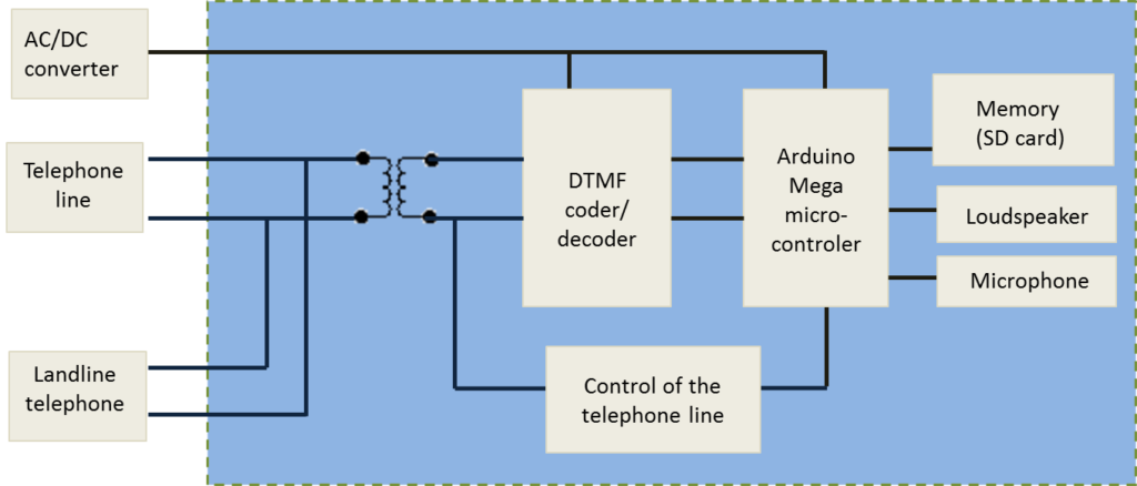
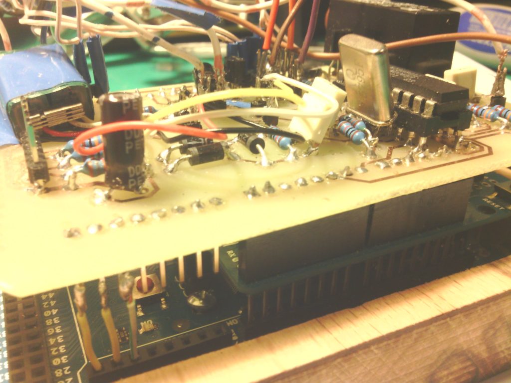
The PCB was designed in Altium Designer software as shown in figure below and produced manualy in a university lab. Some of the phases of development and how does a device looks from inside is shown in figures below too.
. 
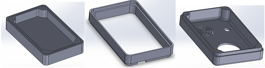
The casing was designed in a Solidworks software and was produced on a CNC milling machine that Youth Research Center (ICM ) owns. Pictures of the model are shown below.
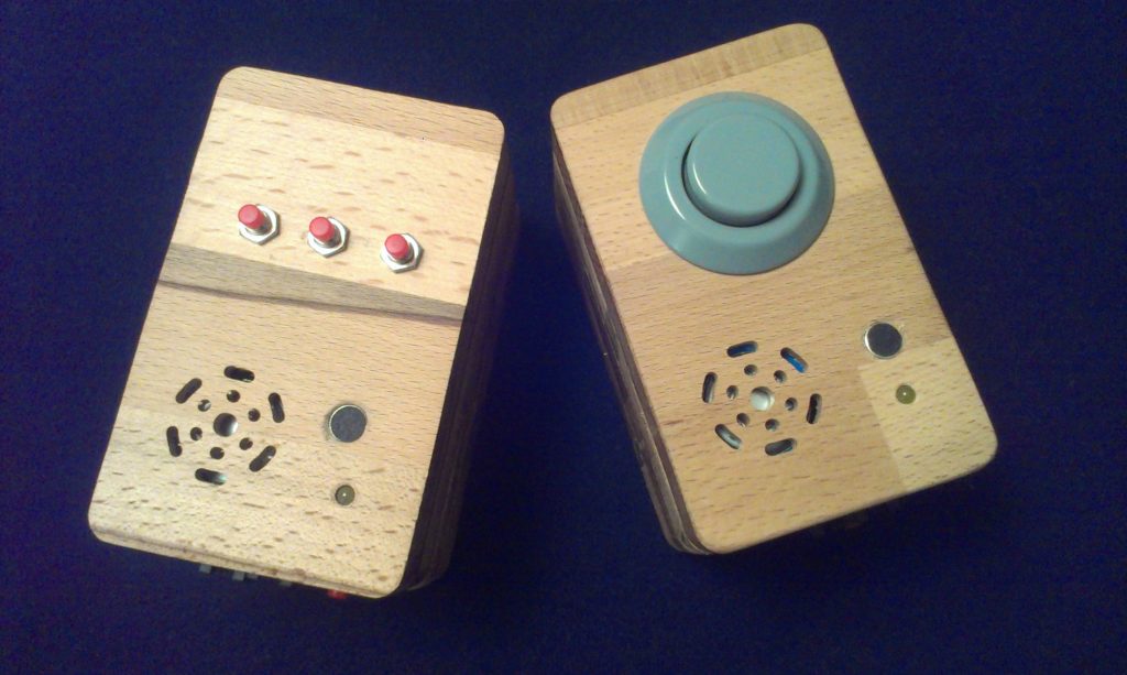
Final device with two versions of interface is shown on figures below.
2.Working principle
Today most telephones use DTMF [4] (Dual Tone Multiple Frequencies) standard, which defines combination of two frequencies that represent particular telephone digit/symbol. All phone devices that support DTMF dialing can generate 12 DTMF signals which represent digits/symbols: 1, 2, …, 9, 0, ‘*’ and ‘#’.
For the realization of proposed solution platform “Arduino” has been chosen, because it is “open source” and relatively cheap. The entire device is designed as a “shield” board which is just stacked on top of the Arduino board. In order to have phonebook that is easily transferable and editable, all contacts and corresponding telephone numbers are written in a single .txt (ASCII) file stored on the SD memory card. The phone numbers in the file are in the following format:
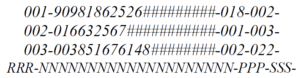
First three digits (RRR) are the number that denotes the name of the file (.wav) where contact name audio recording is stored, but also the number of the row of number in .txt file. 20 characters (NNN…N) are reserved for the telephone number. If the number has less than 20 digits, the rest of the characters are replaced with symbol ‘#’. Last two three-digit numbers represent previous (PPP) and following (SSS) contact (its position in .txt file and the name of the .wav file). In such a way a linked list is created with pointers to next and previous contact.
Device testing
One the device was built and its operability tested, in order to examine functionality and suitability of user interface for the visually impaired, the device was given to blind people to test it. In cooperation with the Croatian association of the blind functionality and user interface was tested by 11 blind or visually impaired users. It was planned to test the device on more people, but not all were able to participate in the available time frame. Six examiners were older than 50 years, and five were younger. Although the group of 11 examiners is relatively a small group from which statistically significant results cannot be obtained, we believe that the homogeneity of the results can confirm quality of functionality of the proposed solution. The review of similar studies with the blind [7-10] revealed that the number of the examiners was also small (under twenty examiners).
More details about the study of testing device can be found in the published paper that is linked below.
The blind examiners have concluded that the device with its interface and functionalities is fully adapted to their needs, and the overall impression was positive. The first hypothesis was confirmed: it is possible to make a device that would help all blind people.
The designed and developed audio phonebook for the blind people can facilitate the usage of the phone for blind. The device solves the main problems that the blind people have when making a phone call: stores a large number of contacts, completely eliminates the risk of dialing the wrong number or being interrupted because of slow dialing. This confirms the second hypothesis.
Several advices for further improvements of the device were collected. The advices were mainly oriented to new functionalities, and not to the modification of existing functionalities or interface. Additional feedback obtained from the examiners indicates the need for a similar user interface on other devices they use in everyday life, which represents a potential market niche at the global level.
Except the feedback on the device itself, a profile of blind people was created, their needs, problems, current solutions. An overview on part of the community of blind people, to whom this device could help, was acquired. Those people are ones who did not manage to get used to the new technologies, especially on touchscreen. To those people the device would not only enable easier dialing of a phone number, but would also solve the problem of need to memorize a lot of contacts. In this research, more than half of the examined people have belonged to that category. This also indicates that the third hypothesis could be confirmed, but a carefully selected group of examiners is required in order to get scientific proof. They might now be able to delete or add new contacts, depending on severity of their cognitive impairment but calling could be obtained.
Acknowledgement
We would like to thank Predrag Pale for the initial idea of the device, as well as for support and help during the work on the project. We also thank the Croatian association of the blind: “Hrvatski savez slijepih i slabovidnih” for assistance in carrying out the tests. Thanks go also to all examiners that participated in the research and tested the device.
For this project Goran Popović and I were awarded with the Rector’s Award (the highest award a student can get at the university) in 2015. We would like to thank to the prof. Hrvoje Džapo who was our mentor for this award. Whole text that was awarded can be seen here (in Croatian): Rectors-paper
The poster from the exhibition of awarded papers can be seen here (unfortunately it is in Croatian too): Rectors-poster
Short student paper about this work was presented on MIPRO conference in Opatija, Croatia in 2016. The paper was published in Proceedings of the 39th International Convention, pp. 1924-1929 and can be downloaded here: MIPRO-paper
Literature
[1] http://www.savez-slijepih.hr/hr/clanak/sljepoca-teskoce-i-dodatni-troskovi-njome-prouzroceni-455/, (7.4.2015.)
[2] http://www.androidcentral.com/what-google-talk-back, (7.3.2015.)
[3] R.Yousef, O.Adwan, M.Abu-leil.“An enhanced mobile phone dialler application for blind and visually impaired people“ , International journal of engineering and technology, 2 (4) (2013) 270-280
[4] D.Nassar. „DTMF Encoding and Decoding“, Circuits (radio electronic), Dec.1986
[5] Arduino Mega 2560: http://www.arduino.cc/en/Main/arduinoBoardMega (12.4.2015.)
[6] MT8880 datasheet: http://pdf1.alldatasheet.com/datasheet-pdf/view/77086/MITEL/MT8880.html (17.4.2015.)
[7] M.Sečujski, D. Pekar. „Evaluacija različitih aspekata kvaliteta sintetizovanog govora“, Fakultet tehničkih nauka Novi Sad; AlfaNum d.o.o., Novi Sad
[8] http://www.savez-slijepih.hr/hr/clanak/ii-metodologija-istrazivanja-1440/ (28.1.2015.)
[9] M.Sečujski. „Ka automatskoj sintaksnoj analizi rečenice na Srpskom jeziku“, Fakultet tehničkih nauka Novi Sad
[10] K. Nenadić. „Relaksacija kao pomoćna metoda peripatološkog programa“, Sveučilište u Zagrebu, Edukacijsko rehaibilitacijski fakultet, 1999.


 Image shows RAMPS board with a newly designed PCB for 2 Arduino Pro Mini and H-bridges.


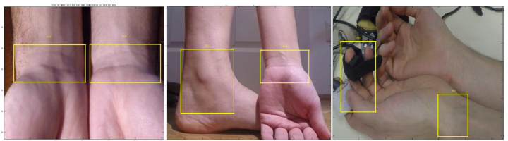
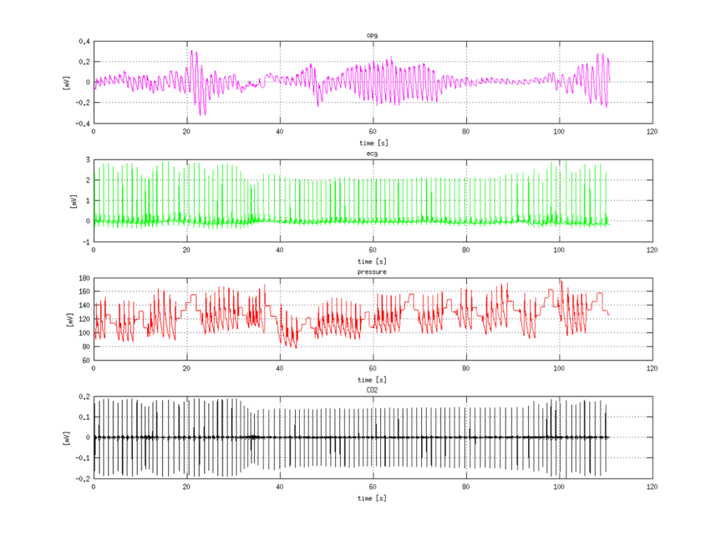
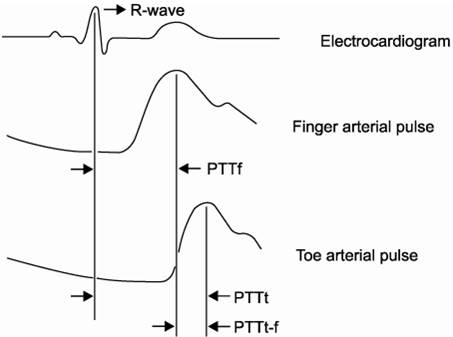
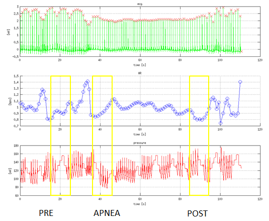
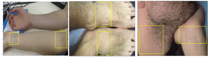 Example of recorded signals is shown on next picture. First signal is photoplethysmogram (PPG), then electrocardiogram (ECG) and third measured is pressure. Fourth signal is CO2 consumption which was not measured but computed, and is not important for the project.