Science and technology are today moving in the direction of automation and autonomy of the systems. Detection of vegetation along the roads is one of a series of ideas that seeks to achieve the autonomy of the vehicles in traffic without the presence of the driver. By analyzing the images of captured environment it is necessary to determine which parts of the image are vegetation, and which are not. Due to the complexity of the problem, deep convolutional neural network which is trained on a large number of examples is used. After that, the goal was to examine the quality of the network on several images that were obtained as a result of the network. In this way it was possible to create a visual impression of the quality of the network.
Introduction
The environment around the vehicle is recorded with the camera. We wanted to be able to determine what parts of the image are vegetation and what is not. This task cannot be achieved only by image analysis because there are too many variations that cannot be formally described. From this reason we moved in the direction of neural networks which are able to recognize patterns on the basis of a large number of examples. In this case, due to the complexity of the task, number of samples is very large (about 500,000). Therefore deep convolution neural network were necessary so that treatment could be in a finite amount of time. Training and testing was performed on GPU in order to reduce processing time needed.
The complexity of the problem lies in the fact that vegetation does not always mean only “green grass”. A large number of variations are possible; eg. different seasons which change vegetation color, the presence of leaves in autumn, shadows, bark of trees, colorful flowers, etc. Also along the curb are often parked cars or the camera captures the people passing by. For this reason, the color is not good enough criterion for identifying the vegetation.
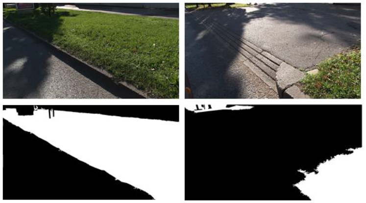
For training the network a large number of images of lots of different situations is needed. For each image manually tagged masks are needed. Masks are the desired output of the network, or one-dimensional black and white image in which the vegetation is designated with1, and the rest is 0. Examples of images and a corresponding mask are shown in figures below.
Deep convolution network
Deep networks are networks with many hidden layers between the input and the output layer. Specifically in this case, we used deep convolution neural networks that operate on the convolution and image compression. The importance of these networks is great as it helps to extract key features to classify each individual pixel.
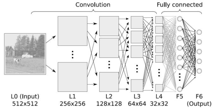
Figure above shows a typical structure of a deep neural network. The entrance can be one monochromatic images or multi-channel color image. Then alternating array of convolutional and pooling (compression) layers follows. At the end are several fully connected layers (classical perceptron) which are two-dimensional (including the output layer). Typical deep convolutional network has around ten layers. Convolution layers and pooling layers have two-dimensional “neurons” that are often called “feature maps” and which in each layer are becoming smaller. The convolutional layers are connected to the previous layers, and adjust connection weights by learning. The pooling layers do not learn any weights.
These networks are easier to be trained than other deep learning methods, and it is also possible to find more features, which can be passed through filters (which are practically layers of deep convolutional neural network). They also require relatively little preprocessing. In some cases, they were shown to work better than a man. But often they are criticized because of poor understanding of what is actually happening inside the hidden layers.
“Caffe” tool
We used the “Cafe” tool. It is a tool that runs the training of deep neural networks instead of us. In order to use “Caffe” tool, we had to adjust the input data in the appropriate format (LMDB). Then the network had to be designed; layers should have been named and sizes and interconnections defined (in .prototxt format). Location of test and validation sets of images had to be linked.
Parameters of training (solver.prototxt) had to be defined. Parameters include: the maximum number of iterations, after how many iterations validation follows, what is the rate of learning, etc. After the training, the network had to be tested.
Preprocessing of images
Two hundred pictures of different scenes were used as a set for training. But first few preprocessing steps were needed in order to obtain the final dataset for training. The image dimensions were 1080×1920 px which is too high and were reduced in both dimensions to the dimensions of 270×480 px.
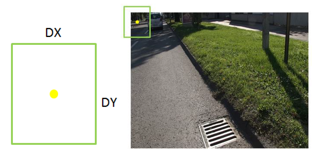
The input to the network is not the whole picture but a cutout frame of DXxDY pixels around the central [cx, cy] pixel. Using DXx DY surrounding pixel networks should conclude whether the central pixel is vegetation or not: there are two possible exits, 1 or 0. For each frame correct answer is also needed in order to train. The correct answer is value of [cx, cy] pixel in the mask image.
In order to improve training, large number of DxxDY frames were cut out from each image and together with correct answer stored in a file in the form:
crops_train / 3_1.jpeg 0
crops_train / 3_2.jpeg 1
…
This format is called LMDB. It is important that the test data consists of approximately the same number of positive and negative examples, and that they are uniformly spaced.
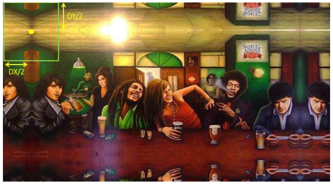
Since the boundary pixels also have to be classified it is necessary to expand the image around them so that there is also DXxDY pixel frame around them. Expanding is done by mirroring: on all edges of the image boundary DX/2 or DY/2 pixels is flipped and the images are stored. Only after this process is done, cutting the frames and converting to the LMDB format is done. All of this is shown in images below.
Since most of the networks are designed for the input data in the range [0,1], and the color values of pixels in the image are in the range [0,255] it was necessary to scale the value of all pixels.
Matlab script was written which performs all preprocessing that was mentioned so far:
– reduces images
– mirrors edges
– scales values to [0,1]
– cuts out frames at random coordinates
– saves frames as a separate files
– gives the names to the frames and stores the result in the LMDB file
Postprocessing and testing
Testing the quality of training networks was done on several images from the test set. Matlab script was written which takes one by one image from the test set, reduces it to 270×480 px, scales values to [0,1], extends in the same manner as in the preprocessing, and then for each pixel cuts out a frame and sends into a neural network.
Network gives as a result two numbers; the probability that this pixel is 1 (vegetation), and the probability that the score is 0 (Others). After the results of the network, it is necessary to determine the threshold above which the percentage will determine whether it is vegetation or is not. Determination of percentages is done using ROC curves.
When threshold is defined, it is finally decided whether the network said 0 or 1 for each pixel. After that the resulting image is constructed. Visually it is possible to compare the resulting image and corresponding mask which represents the exact solution.
To determine the numerical accuracy of the network, this process is repeated for several pictures and in each image it is calculated as the number of exactly classified pixel values. Accuracy is calculated for each image, and finally evaluated to get the average accuracy of all images. All this is recorded in the .txt file.
Results
In trying to evaluate the work of each of proven neural network using MATLAB wrappers for Cafe for every given input (cut out the frame around [cx, cy] pixel images for testing), we got the same output from the network. We tried to solve this problem on different ways which included the review of everything done so far.
First we changed the architecture of the network several times, but each time the problem remained present. Then we tried the scaling of the input data to the interval [0,1]. Then we noticed that other people(from the Internet) reported the same problem , and we tried to apply the advice which they suggested, and that was the reduction of learning and mixing together for training, but even that did not help.
The last attempt was balancing the training set in a way that has exactly 50% of the positive examples for learning. Previously training set was created by randomly cutting out the frames from the images, ignoring their label, so the result was a significantly higher number of negative training examples. Training of these data with a rate of 0.0001 teachings caused the loss function through iteration learning slightly oscillates around the value of 0.70 from which we assumed that that was a local minimum from which with such a low rate of learning, function loss could not move. However, increasing the learning rate to 0.1 and then after training, network function loss slightly decreased, but still oscillated.
Conclusion
We examined the deep convolutional neural networks and designed several of them in an attempt to resolve the problem of detection of vegetation along the roads.
Matlab scripts for pre- and post-image processing were constructed. Preprocessing performed certain operations on the input images and created a data set for training and validation. Post processing takes the entire image and part by part (frame by frame) receives the result of the network. The goal is that these results match as good as possible with the corresponding mask, and thus except from the numerical accuracy of the network and visual the quality of a network.
Unfortunately, the final structure of the network that successfully detects vegetation has not yet been found. There were problems that the loss function during training network does not fall continuously but oscillate. Also after the end of training, when the testing is performed, it returns almost the same value for each input frame, and gives the same result regardless of the input.
Work on the problem will continue.
Acknowledgement
This project was a project on a Neural networks course and was done in a group of three students: Toni Antunović, Mladen Kukulić and me. The final report can be seen here (in Croatian unfortunately): Project-text and the presentation (in English) here: Project-presentation.
Literature
- „Raspoznavanje objekata dubokim neuronskim mrežama“, Vedran Vukotić, Diplomski rad, FER 2014
- „Caffe: Convolutional Architecture for Fast Feature Embedding“, Yangqing Jia_, E. Shelhamer, Donahue, S. Karayev, UC Berkley
- http://caffe.berkeleyvision.org/ (access 20.12.2014.)