
Heart rate variability
Heart rate variability (HRV) refers to the variation of the intervals between consecutive heartbeats over time.
It is indicator of many physiological processes taking place inside of the body since it is being controlled by regulatory mechanisms of autonomic nervous system which reacts immediately to any physiological state. Too static HRV is indicator that regulatory mechanisms are not working properly and that something wrong is happening with organism.
Heart rate is regulated by sympathetic and parasympathetic input to the sinoatrial node. Sympathetic nervous system (SNS) by releasing hormones increases heart rate and thus controls some extreme situations. On the other hand parasympathetic nervous system (PNS) controls routine functions of the body and mainly decreases heart rate. As a consequence continuous interplay of SNS and PNS can be measured by the HRV.
Frequency spectrum
As just explained above it is normal that HR changes in time, but the speed of changes (HRV) is what is very interesting to observe. Frequencies of HRV are separated in three bands, high, low and ultra-low as specified in table below.
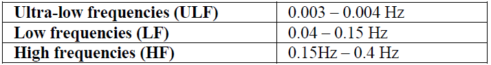
It was shown that PNS is related with power of HF band and indicates short-term regulatory mechanisms, while on the other hand SNS activity (and sometimes PNS) is related with power of LF band and indicates mid-term regulatory mechanisms. ULF band is related to very slow oscillations and indicates long-term regulatory mechanisms. [1] SNS activation presents as slow increase of HR meaning also reduction in HRV, while PNS activation indicates as fast decrease of HR and increase in HRV.
Increased activation of SNS can be caused by stress, physical activity, standing, 90˚ tilt ect. while activation of PNS can be attained by controlled respiration, cold stimulation of the face or rotational stimuli [6.]. Physical exhaustion is indicated both by decrease in PNS and increase in SNS, while on the other side positive stress is indicated as increase in both PNS and SNS. SNS plays important role in causes of arrhythmias and PNS reduces possibilities of arrhythmias thus having protective role. Altogether, PNS activity is sign of healthier people, while its reduced activity can indicate some type of dysfunction.
Wavelet transform
Today’s most common analysis methods of HRV are spectral analysis techniques using the Fourier transform, which assumes that the signal is periodical in time. Problem with such techniques is lack of temporal resolution. To overcome this limitation, time window frames are often used, so that small segments of the signal are analyzed, for example as in Short time Fourier transform (STFT). However, time-frequency resolution depends on the width of the window used. As a consequence, higher temporal resolution means lower frequency resolution and vice versa. From this reason Wavelet transform as a method which performs time- frequency analysis of non-periodic signal is studied.
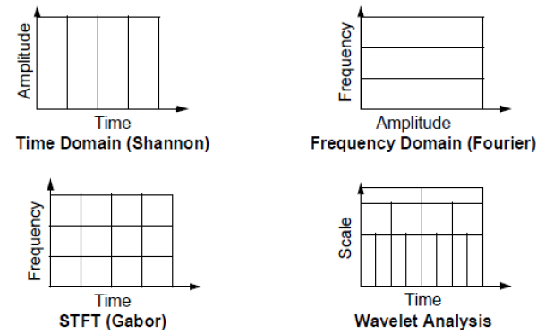
Wavelet analysis allows the use of long time intervals where we want to observe more precise low frequency information, and shorter regions where we want to observe high frequency information. In figure above comparison of FFT, STFT and WT is graphically represented.
Wavelet transform name comes from the fact that it uses a waveform instead of sinusoid function used in Fourier transform. Mother wavelet is waveform of effectively limited duration that has an average value of zero. Wavelet analysis does not use a time-frequency region, but rather a time-scale region. This is because wavelet analysis works by breaking up a signal into shifted and scaled versions of the mother wavelet. Scaling a wavelet means stretching (or compressing) it, where small scale is very compressed signal and large scale is stretched signal. Scale is related to the frequency of the signal in a way that smaller scale means larger frequency and vice versa. Shifting wavelet means delaying it in time. Wavelet transform works in a way that mother wavelet is compared sequentially to sections of the original signal. The result is set of coefficients that are a function of scale and position. These coefficients can be represented and used in many ways. In some cases, inverse transform can be done, which enables to reconstruct signal using only this coefficients.
There are three types of wavelet transform that a commonly used: continuous wavelet transform (CWT), continuous wavelet transform using FFT (CWTFT) and discrete wavelet transform (DWT). Some of the most important properties of each are listed below.
1.Continuous wavelet transform – CWT
In continuous wavelet transform correlation of signal with mother wavelet can be calculated for any scale and shift of mother wavelet. CWT is calculated in a way that scaled wavelet function is shifted smoothly along the signal and correlation with that signal section is measured.
2. Continuous wavelet transform using FFT – CWTFT
Problem with CWT is that it is redundant and there is no unique way to define inverse. This means that it is not possible to reconstruct signal from coefficients. CWTFT uses FFT of the wavelet function in order to reconstruct signal. Not all wavelet functions can be used in CWTFT. Condition is that it is real value function and that its FFT has support on only positive frequencies. Wavelets that satisfy this admissibility condition are called analytical wavelets.
3. Discrete wavelet transform -DWT
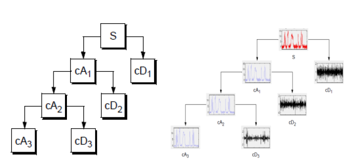
In order to speed up calculation, discrete wavelet transform is used. In DWT “dyadic” (which means based on factor two) scales are used. Even though only few scales are used to cover the whole area of frequencies, transform is much more efficient and equally accurate. In each level of transform signal is decomposed on “detail” and “approximation”. Details are low scale (high frequency) components of signal, while approximations are high scale (low frequency). In each consecutive level approximation is decomposed into detail and new approximation whose scale is smaller and frequency is larger. Iteration of this process results in wavelet decomposition tree. Example of one decomposition tree is shown in figure below. This process could be continued indefinitely in theory, but in practice it is limited with the resolution of the signal. When individual detail consists of a single sample, the end level of decomposition is reached.
Project idea
There is a large repository of papers that were interested in wavelet transform itself and its application on HRV evaluation. It is clear that this is very interesting area and that this technique could further improve understanding of the interactions of the autonomic control systems with the cardiovascular system. In this project idea was to investigate through different approaches which type of wavelet transform is the most appropriate for HRV analysis and what are all the parameters that influence the speed, quality, resolution etc. of the decomposition. Therefore the results of this paper might serve as starting point or component of some future research.
Analysis of wavelet transforms
1.Comparison of methods
Idea was to analyze mentioned three methods of wavelet transform in order to compare them, detect what advantages and drawbacks of each are and to choose the best one on which HRV analysis will be further studied. Several methods were tried; pure coefficients comparison, reconstructed signal comparison, sum of coefficients for each of frequency band of interest (ULF, LF and HF), energy distribution and calculation time comparison.
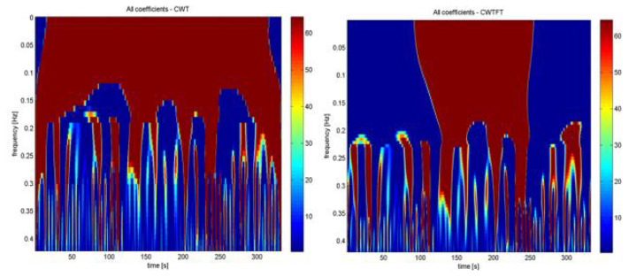
Pure coefficients were compared only for CWT and CWTFT since DWT has only few scale levels. In HF frequency range there is almost no difference between CWT and CWTFT, but as approaching to ULF frequencies differences increase as can be seen in figures below. Unfortunately, appropriate explanation for that was not found but it is believed that it is because of some constraints of CWT for very low frequencies. Also some differences could be caused by slightly different boundary frequencies for frequency bands.
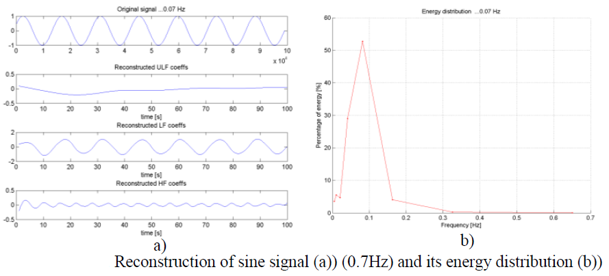
For comparison of reconstructed signals, original signal was reconstructed using coefficients for each frequency band separately. This was only possible to do with CWTFT and DWT method. Again, difference was very small for HF and LF, only for ultra-low frequencies (UFL) difference was more visible, but even then main trends were the same.
In order to compare all three methods at the same time, sum of all coefficients for every frequency band was studied. Results are very similar for all three methods with only minor differences for HF and LF band. For ULF band larger difference for CWT is noticed which agrees with previous results.
Distribution of energy through different frequencies was studied in order to compare methods with Fourier decomposition of signal. The results have shown very good correlation between frequency values of peaks of energy distribution and FFT spectrum.
The last thing to consider was computation time for different methods. CWT method consumes very much time and CPU power. CWTFT takes only few (< 5min) minutes to compute even for signals with almost million samples in comparison to CWT which takes few hours (<3h) for the same task. On the other hand DWT is even faster than CWTFT and it takes under minute to do the decomposition.
Conclusion is that DWT is the best method for the wavelet decomposition for several reasons: time and CPU power consumption, simplicity of decomposition and reconstruction and the quality of decomposition and reconstruction itself.
2.DWT method analysis
1) Quality of decomposition
Quality of decomposition was tested using artificial sinusoidal signals of known frequencies. Frequencies within different frequency bands were used. Energy distribution globally and how well the peak of maximal energy corresponds to the frequency of sinusoid was studied. Reconstruction signals using separately HF, LF and ULF frequency bands ware observed (their amplitude and period) too and is shown on figures below. Detection to which band some frequency belongs, based on reconstruction is precisely detected only for frequencies which are in the middle of the frequency band and further from the boundaries. As getting closer to the boundaries other bands detect these frequencies too, but with lower amplitude and wrong period. Also quality of detection based on energy distribution depends whether the frequency is closer or further from one of the frequencies corresponding to the scales that were used in decomposition (since DWT uses dyadic scales). Frequency detection was very precise for ULF and LF band, but less precise for HF band, since for them frequencies resolution is smaller and the error is larger.
2) Noise influence
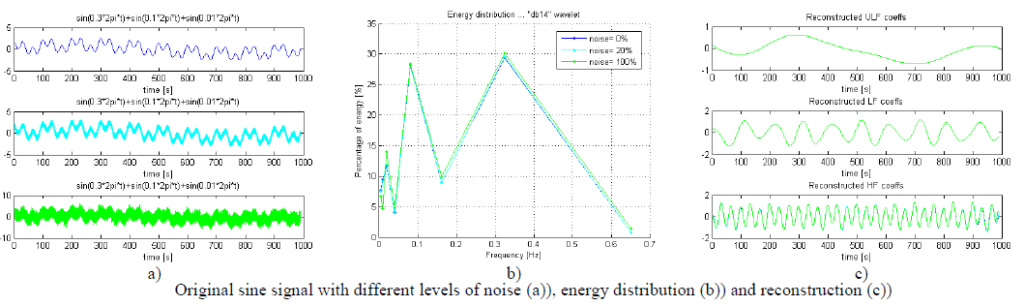
Signal which consists of sinusoid waves of three different frequencies (each within one frequency band) was used. To this signal two different levels of Gaussian noise were added. Reconstruction and energy distribution for signal with and without noise was studied and is shown on figures below.
Results showed that noise didn’t influence decomposition and reconstruction even when amplitude of noise was in range of signal amplitude. This is another very positive property of DWT transform.
3) Influence of chosen wavelet function
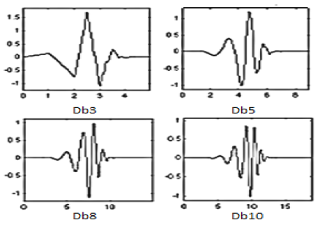
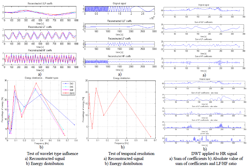
Finally, the influence of chosen mother wavelet function on energy distribution and reconstruction was studied. Four wavelets from Daubechie’s family were used: “db3”, “db5”, “db8” and “db10” as shown in figure below. Result of comparison is that difference is very small for LF and HF band, but for ULF there are noticeable differences. For LF and HF, reconstruction signals look very similar especially for “larger” Daubechie wavelet functions (shown in figure below). It is because larger orders of Daubechie functions are more complex ones, but also more similar to each other than the ones of small order (for example Db1 is actually step function). For this reason for precise calculation it is suggested to use enough large Db wavelet function (>Db8). Last thing to notice is that reconstructed signals in each band are not sinusoid functions as one may expect. This is due to the fact that borders of frequency bands in DWT are not very precise.
4) Temporal resolution
Signal whose frequency content changes in time was used. First part of the signal is sinusoid with frequency of 0.3Hz which is in HF band, then sinusoid of 0.1Hz (LF band) follows and at the end sinusoid of 0.01Hz (ULF band). It can be seen from reconstruction signals for different frequency bands that time detection of each sinusoid within input signal is very precise (shown in figure below). Also energy distribution clearly shows peaks on frequencies values of original signal. This confirms DWT ability to analyze signal in frequency and time domain.
Analysis of HRV using wavelet transform
Five minute signal of heart rate sampled with 500 sample/s is used to present input and output data of HRV analysis using DWT method. In figure above original signal and DWT coefficients separately for ULF; LF and HF frequency band are presented.
As previously mentioned, parasympathetic nervous system (PNS) is major contributor to HF component. Slight disagreement exists in respect to the LF component. Some studies suggest that LF is a quantitative marker of sympathetic (SNS) activity, while other studies view LF as reflecting both sympathetic and parasympathetic activity. Consequently, the LF/HF ratio is sometimes introduced to mirror sympathetic-parasympathetic balance and also to reflect the sympathetic modulations.
LF/HF ratio is obtained by dividing values of LF coefficients with HF coefficients. Absolute value is used because we are interested in “power” of the LF and HF band in time. After division, LF/HF ratio was averaged in time using median filter with a window size of 500 samples which corresponds to one second. This way resolution of LF/HF ration is one second which is reasonable. In order to visually better see connection between LF, HF coefficients and LF/HF ratio in figure above, absolute values of coefficients are plotted.
In this signal HRV during respiration is observed. Such, deep breathing or apnea, tests are usually used in clinical testing or calibrations. During normal uncontrolled breathing respiration seems to influence HRV for less than 10%, but controlled respiration increases this influence up to almost 50% [3.]. During apnea or suspension of breathing, heart rate changes with frequencies in range from 0.01 to 0.04 Hz. This means that power of ULF band of HRV increases. Also at the same time LF/HF ratio is increased [4.] as a consequence of higher sympathetic processes. Similar effect happens during sleep of patients with sleep disordered breathing, where increased LF/HF ratio reflects not only sympathetic dominance but also reduced parasympathetic control [4.]. In the signal on figure above it can be noticed that LF/HF ratio is increased in time between approximately 130th and 230th second. In the same time interval ULF coefficients values are relatively large in comparison to the rest of the time. These two things indicate that at this time interval patient might have suppressed breathing. This could be confirmed if breathing was also recorded at the same time.
Conclusion
In this work, possibility to analyze heart rate variability (HRV) with wavelet transform was investigated. Three methods of wavelet transform were compared (CWT, CWTFT and DWT). Since, DWT showed to be the best one from several reasons: time and CPU power consumption, simplicity of decomposition and reconstruction and in the end quality, it was tested further. Quality of DWT decomposition, noise influence, mother wavelet type influence and time resolution were observed. DWT showed to have high noise robustness, excellent temporal and good frequency resolution, and as such showed to be very good candidate for more precise analyses and someday even usage for other scientific and clinical purposes.
Acknowledgement
This work was done during Erasmus+ exchange on Technical University of Vienna. I would like to thank to my two mentors that gave me opportunity to work on this project and helped me all the way along F.T. and E.K. Short report can be downloaded here: BSS_report
Short student paper about this work was presented on MIPRO conference in Opatija, Croatia in 2016. The paper was published in Proceedings of the 39th International Convention, pp. 1930-1935 and can be downloaded here: MIPRO_paper
Literature
[1.] E. Kaniusas: Biomedical sensors and signals I, Springer 2012.
[2.] Task Force of the European society of cardiology and the North American society of pacing and electrophysiology: Heart rate variability – Standards of measurement, physiological interpretation, and clinical use, European Heart Journal, 1996
[3.] V. Demchenko,R. Čmejla, J. Vokřál: Analysis of heart rate variability during respiration
[4.] I. Szollosi, H. Krum, D. Kaye, M. T. Naughton: Sleep Apnea in Heart Failure Increases Heart Rate Variability and Sympathetic Dominance, Sleep Journal, 2007.